There is more than one aim in our calculations. First, we want to be
able to calculate amplitude spectra of oscillations. In Fig. 1
we show for l=1 to l=4 the normalized amplitude spectra (which are
independent, for small amplitudes, of the often unknown inclination
i; e.g., RKN, BFW). As one can see from Fig. 1, the slope
varies strongly with l. By comparing the observed slope with the
theoretical slope, one can therefore determine l (the slope also
depends on ![]() and
and ![]() , which may have to be
constrained from other observations).
, which may have to be
constrained from other observations).
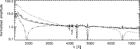
Figure:
Normalized amplitude spectra for l=1 (solid), l=2 (dashed), l=3
(dotted) and l=4 (dash-dotted) modes ( ![]() ,
,
![]() ,
, ![]() ). Around 1900 Å the phase of the l=4
mode changes by
). Around 1900 Å the phase of the l=4
mode changes by ![]() , causing the amplitude to go to zero
, causing the amplitude to go to zero
A second aim of our program is to calculate time-resolved
spectra. This is shown in Fig. 2 for l=1, m=0 for a strong
oscillation resulting in variations of ![]() of
of ![]() .
One can see that the spectra depend strongly on the
inclination. Furthermore, one can see the effects of having a
distribution of
.
One can see that the spectra depend strongly on the
inclination. Furthermore, one can see the effects of having a
distribution of ![]() at maximum and minimum instead of a
uniform
at maximum and minimum instead of a
uniform ![]() across the WD surface.
across the WD surface.
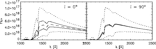
Figure 2:
UV-spectra at maximum and minimum (solid) for l=1, m=0
oscillations with ![]() for
for ![]() (left) and
(left) and ![]() (right). Also shown are the equilibrium spectrum
(
(right). Also shown are the equilibrium spectrum
( ![]() ,
, ![]() ,
, ![]() ;
dashed) and spectra at
;
dashed) and spectra at ![]() (dotted)
(dotted)
A third aim is to properly take into account non-linear variations of
I with linear, i.e., sinusoidal, variations of ![]() . For
the above case we show in Fig. 3 the light curve for a filter
located near the center of
. For
the above case we show in Fig. 3 the light curve for a filter
located near the center of ![]() and just outside this
line. One can see that the light curve differs strongest from the
underlying pure sinusoidal variation of
and just outside this
line. One can see that the light curve differs strongest from the
underlying pure sinusoidal variation of ![]() near the center
of the spectral line. This causes strong amplitudes at higher
harmonics in the Fourier spectrum.
near the center
of the spectral line. This causes strong amplitudes at higher
harmonics in the Fourier spectrum.
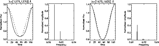
Figure 3:
Light curves and corresponding Fourier spectra for oscillations as in
Fig. 2 with ![]() close to the center of the
close to the center of the ![]() line (left panels) and just outside the
line (left panels) and just outside the ![]() line (right
panels). The underlying sinusoidal variation of
line (right
panels). The underlying sinusoidal variation of ![]() is
overplotted (dotted)
is
overplotted (dotted)