This star is of great interest since it may well define the blue edge
of the ZZ Ceti instability strip, which depends strongly on the
a-priori unknown parametrization of the MLT (e.g., Bergeron et
al. 1992). G 226-29 was observed with the HST using the FOS. Five
observing runs were made, each about three hours long. The individual
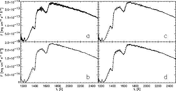
exposure times were about 9 s. Figure 4a shows the average
spectra of the individual runs (these are corrected for a
wavelength-dependent light loss modulated with the HST orbital
period). Near about 1500 Å differences between the runs
appear. However, the spectrum averaged over all runs (Fig. 4b)
can be assumed to not be affected by this (it is also hardly affected
by the light loss). We therefore fit this spectrum and obtain an
average ![]() (the error is dominated by systematic
errors which are hard to estimate) at
(the error is dominated by systematic
errors which are hard to estimate) at ![]() (the latter
adopted from Koester et al. 1996) using the
(the latter
adopted from Koester et al. 1996) using the ![]() MLT,
MLT,
![]() , l=1 and
, l=1 and ![]() . The latter two parameters
were adopted from results of WET observations by Kepler et al. (1995).
These observations showed one triplet in the Fourier spectrum. It
should be noted, however, that this interpretation of the triplet is
not the only one possible. We exclude in the fit the region above
about 2300 Å where the observed slope changes. This is
evident also in other HST spectra and indicates some calibration
problem. The high signal-to-noise HST spectrum reveals differences
between observations and theory. These could be caused by continuing
calibration problems, an imperfect line broadening theory for
. The latter two parameters
were adopted from results of WET observations by Kepler et al. (1995).
These observations showed one triplet in the Fourier spectrum. It
should be noted, however, that this interpretation of the triplet is
not the only one possible. We exclude in the fit the region above
about 2300 Å where the observed slope changes. This is
evident also in other HST spectra and indicates some calibration
problem. The high signal-to-noise HST spectrum reveals differences
between observations and theory. These could be caused by continuing
calibration problems, an imperfect line broadening theory for
![]() , an imperfect description of convection or a combination
of those. Finally, we fit in Figs. 4c and d the average maximum
and minimum spectra. A good fit is obtained indicating that
, an imperfect description of convection or a combination
of those. Finally, we fit in Figs. 4c and d the average maximum
and minimum spectra. A good fit is obtained indicating that ![]() varies on the WD surface by up to
varies on the WD surface by up to ![]() .
.

Figure:
HST spectra of G 226-29. (a) average spectra of the 5 runs corrected
for light losses. (b) spectrum averaged over all runs. (c) spectrum
averaged at phases near maxima. (d) spectrum averaged at phases near
minima. In (b) to (d) a fit is overplotted (dotted) using ![]() ,
, ![]() ,
, ![]() , l=1,
, l=1,
![]() and an amplitude such that
and an amplitude such that
![]()